Model description

Economics of fleet segments

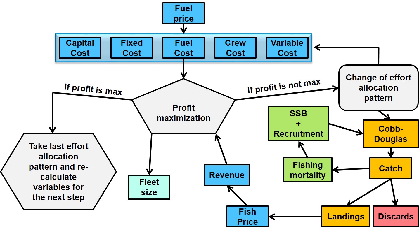
In the economic submodule, gross revenues for each fleet segment are calculated considering landings values of modelled species and also the landings value that comes from catches of other not explicitly modelled species (as fixed percentage). Landings are the difference between catch and discards, whereas discard consists of over-quota catch and catch of undersized species (defined as a fixed proportion of the total catch). Net profit of a fleet segment is calculated as the gross revenue minus all economic costs (fuel costs, variable costs, crew costs, capital costs, and fixed costs. In the model, there is a differentiation between between fixed and variable costs. Fixed costs include vessels costs(such as administrative costs, insurance, and maintenance costs)and are directly proportional to the number of vessels, while variable costs are dynamic and are associated with variations in fishing effort. Fuel costs vary directly with effort. They represent the most relevant cost item in fishing activities for most European fleets. Capital costs involving depreciation and interest payments are defined as a fixed share of the number of vessels. To calibrate the economic submodule, data from the  Annual Economic Reports on the EU Fishing Fleet are used.

Fishers' behaviour

In the model, profit is the main driver of fishers’ behaviour and the aim is to maximize the annual profit for the entire fleet. Thereby,profit depends on the amount of landed fish, prices for the landed fish, and the costs of fishing. Profit, furthermore, depends on the interest rate for capital invested in the fleet. In particular, profit from two years ago determines the level of investment or disinvestment in the fleet, involving changes in the number of vessels of a fleet segment. At the end of each modelling year, the applied CONOPT solver selects a certain effort pattern (number of fishing days and its spatio-temporal distribution) within the historical minimum and maximum that has been observed for modelled fleet segments. This effort pattern is used in the catch function,  a Cobb–Douglas production function, and with regard to the cost, revenue, and profit functions. The effort pattern that results in the maximum annual profit of the entire fleet is then used to calculate the variables for the next time-step. If the solver finds more than one optimal effort, the lower effort level is used. Moreover, this optimal effort pattern impacts the development of commercial fish stocks.

Population dynamics

The optimal fishing effort used in the Cobb–Douglas production function provides a catch estimate, which is then used in Pope’s approximation to calculate the number of individuals. In turn, the estimated number of individuals is then used to calculate the age-specific instantaneous fishing mortality. In the model, individual fish grows according to the von Bertalanffy weight-at-age function. Once a year, stochastic recruitment is calculated via various stock recruitment functions (e.g. Beverton and Holt, hockey stick, segmented regression). Each time the stochastic recruitment model is employed, 1000 stochastic iterations are run. This means that for each time-step per year, 1000 random iterations from the probability distribution in the stock–recruitment function are run.  At the end of each year, all fish of a certain age are moved to the next age class. All fish older than the maximum age are accumulated in the last age class (plus group).